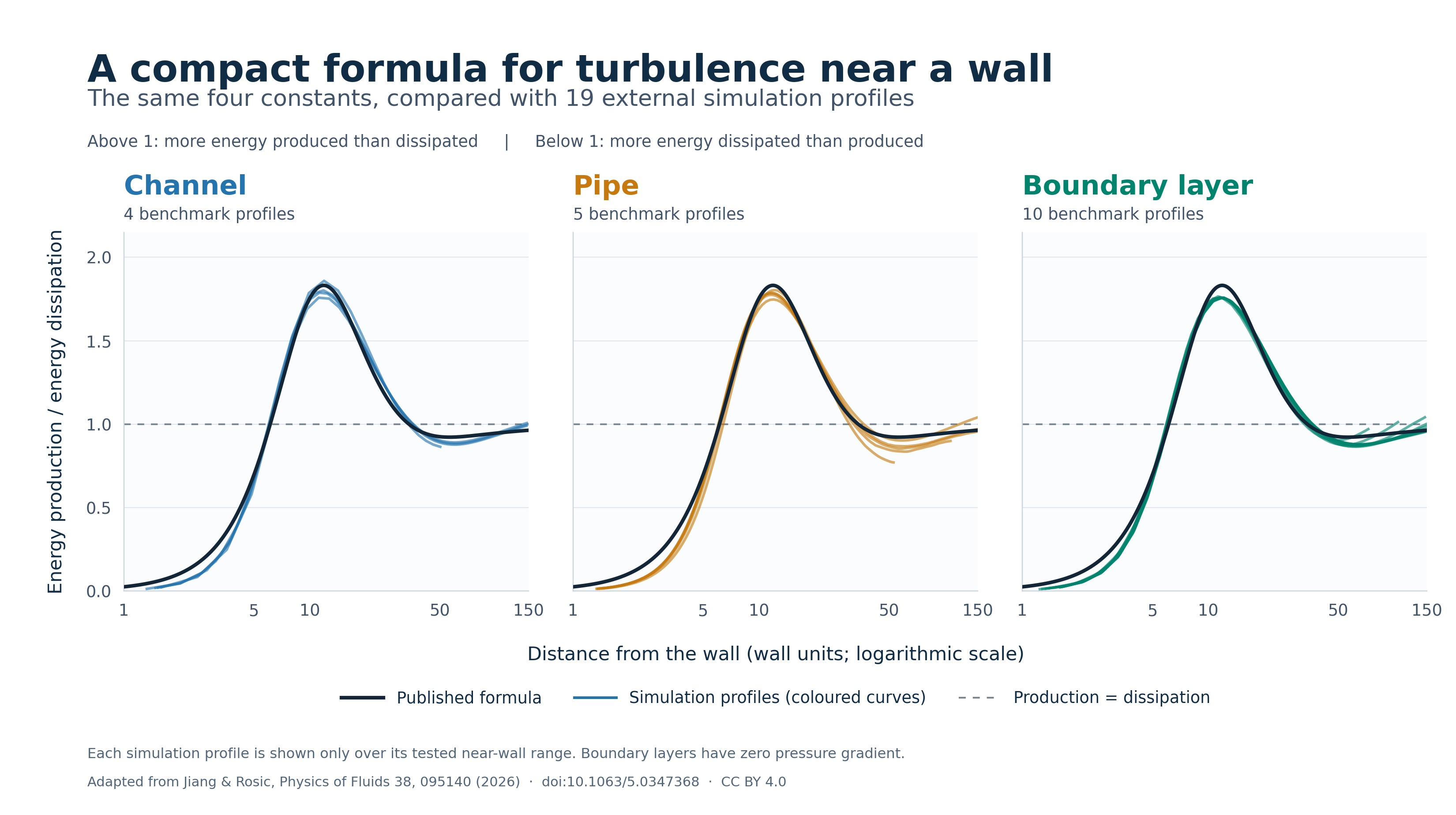
Oxford engineers used symbolic regression and fluid physics to reduce a difficult near-wall turbulence balance to a formula with four fitted constants. The expression followed 19 comparison profiles across channel, pipe and boundary-layer simulations without refitting.
Turbulent flow gains energy from the main current and loses it as that motion dissipates into heat. Many models treat those rates as roughly equal away from a surface. Close to a wall, however, detailed simulations show that production and dissipation separate, making the balance harder to represent with a short equation.
Finding a compact equation
Jianou Jiang and Budimir Rosic of the University of Oxford combined physical analysis with symbolic regression, a machine-learning method that searches for mathematical expressions. They fitted the resulting equation to channel-flow simulations. Its input is distance from a smooth wall in wall units, a scale set by fluid viscosity and friction at the wall. Its output is the ratio of turbulent-energy production to dissipation.
The recommended expression uses four fitted constants. It applies to incompressible, pressure-driven flow over a smooth wall within a stated near-wall domain: greater than one wall unit and no farther than the smaller of 150 wall units or 30 percent of the friction Reynolds number. The friction Reynolds number expresses the flow's size on that same near-wall scale. These bounds restrict the formula to a thin region beside the wall, not the entire flow field.
Testing the formula on other flows
After fixing the constants, the researchers evaluated the equation against 19 profiles from four external simulation codes: four channel cases, five pipe cases and 10 zero-pressure-gradient boundary-layer cases. The boundary-layer cases extend the comparison beyond pressure-driven channel and pipe geometries. The researchers did not refit the constants for each flow type. The same curve followed the tested production-to-dissipation profiles through their intended near-wall ranges.
In a separate dissipation diagnostic, the formula reduced root-mean-square error by 88 to 95 percent relative to assuming equal production and dissipation. That comparison measures reconstruction of the tested simulation budgets. It is not a speedup or accuracy result from a complete computational-fluid-dynamics solver.
The comparison is also broader than the fitting set without being a fully blind test. The Oxford technical note says most of the 19 profiles had appeared during earlier model selection. Training profiles were excluded from the displayed comparison, as were adverse-pressure-gradient and plane-Couette stress tests.
Where the equation stops working
Accuracy worsens when pressure rises strongly in the direction of flow. The expression also does not describe the outer region far from the wall, and it fails outside its stated domain for plane Couette flow, where walls moving relative to one another drive the fluid. Whether inserting it into a full engineering simulation improves predictions or computing cost remains untested.
The equation provides a compact reference for checking near-wall energy budgets and comparing turbulence models. The authors released a NumPy implementation, a short tutorial, frozen evaluation records and checksums under an MIT license, so other researchers can examine the equation without rerunning the symbolic search.
Sources
- Physics of Fluids: Combining symbolic regression and turbulence physics to develop a compact inner-layer production-dissipation closure
- Author repository: formula, code, evaluation records and limitations
- University of Oxford: result summary, technical note and lead graphic
- Lead graphic credit: adapted by Oxford from Jiang and Rosic, Physics of Fluids 38, 095140 (2026), CC BY 4.0